Introduction
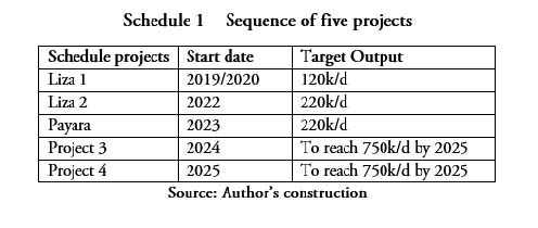
As promised last week, today’s column begins with my presentation of a simple schedule depicting the sequencing of the five projects of ExxonMobil and its partners around which the IDB has modeled Guyana’s oil and gas sector to 2025 in its recent report, ‘Traversing a Slippery Slope: Guyana’s Oil Opportunity, 2020.’ The schedule is intended solely for readers’ convenience, as I have already provided a narrative description of the data last week.
It should be recognized that, explicitly and implicitly, the IDB’s modeling exercise does not provide for: 1) any crude oil production scheduled to come onstream beyond 2025; 2) any other oil projects coming onstream in Guyana before 2025; 3) the prevailing PSA to be substantially modified before 2025; and that 4) Exxon Mobil and its partners remain as the leading international oil company (IOC) producing contractor.
 Together, the five projects aim to produce 750,000 barrels of crude per day by 2025, based on estimated recoverable reserves of around 9 billion barrels of crude oil. The first three projects to come onstream are Liza1, Liza2, and Payara. These aim to contribute 120, 220, and 220 thousand barrels of crude oil per day, respectively, for a total of 560,000 barrels per day. The fourth and fifth sequenced projects are not yet named but are expected to have similar characteristics to those of Liza 1 and to contribute the difference of 190,000 barrels per day required to reach 750,000 per day. The project life, as noted last week, is 20 years with a two-year de-commissioning period.
Following last week’s presentation of the model’s assumptions provided in the IDB’s Note, the next section reports on the model’s parameters as presented therein.
Model Parameters
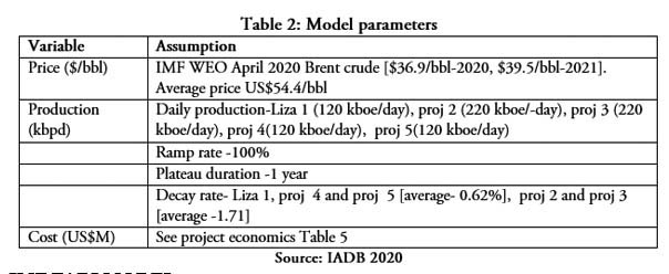
The IDB Note clearly states the model it employs “is built utilizing the cost parameters of the IMF’S Fiscal Analysis of Resource Industries (FARI) model.” It goes on to claim several adjustments to the FARI model. These include: 1) the project characteristics as described above; 2) crude oil price data obtained from the IMF’s World Economic Outlook April 2020; and 3) values are presented in adjusted net present value terms (APV). Several other adjustments were provided as assumptions last week; for example, the ramp rate, the decay rate and the plateau duration.
Readers should note that the IDB has indicated its preference for use of the APV value term because, as it argues, “it is sensitive to the valuation of financial flows for projects with high variability and uncertainty.” Schedule 2 replicates Table 2 (page 21 in the IDB Note) which specifies the model parameters it utilized. Most of these data were discussed last week and the cost data will be presented next week.
IMF FARI MODEL
I devote the remainder of today’s column towards briefly drawing attention to a few key features of the IMF, FARI model, which the IDB’s Note, as indicated here, is built upon.
First, the FARI model is purpose built for natural resources industries and not only crude oil. Second, when applied to the crude oil sector it is constructed around four standard sequential stages of the sector’s project cycle. To recall, these are the exploration, development, production and de-commissioning/closure stages, respectively. Third, the model is typically constructed at the individual project level.
Fourth, it is an Excel- based discounted cash flow (DCF) model. Its framework is designed to measure discounted net cash flows to a project based on a given period (annual!), pre and post -tax; fiscal projections and income flows to the project investors and their respective shares; along with standard measures such as the marginal effective tax rate (METR), internal rate of return (IRR), and average effective tax rate (AETR).
Fifth, there are four key datasets which are required to be inputted to the model. These are: 1) the project characteristics, outlined above; 2) the economic parameters like production, costs, and prices; 3) the mechanisms of the fiscal regime, as detailed in my first column on the topic; and 4) finance, the applicable interest and discount rate.
Finally, it is clear that the IMF FARI model is designed to calculate government take at the project level based upon its applicable accounting rules and specified tax payment obligations. These payments are computed to generate government revenues. A logical extension of this is its utility for revenue forecasting.
Conclusion
I continue consideration of the model next week.